The Recession Spike-and-Revert: Polymarket's Fear Gauge Hit 44.5¢ Last Night and Already Snapped Back
Polymarket's US recession market spiked to an all-time high of 44.5¢ at 22:00 UTC on April 7 — on 12M volume, the lightest day in weeks. It reversed to 29.5¢ within 20 hours. This is the second identical pattern in five weeks.

At 22:00 UTC on April 7, Polymarket's "US Recession by End of 2026" market hit 44.5¢ — an all-time high for the contract. By 18:00 UTC today, it was trading at 29.5¢. That's a 15-cent round trip in under 20 hours.
This wasn't the first time. On March 9, the same market spiked to 42¢ and reversed to 28.5¢ within 24 hours. In both cases, the spike happened on thin volume, at roughly the same time of night, and the reversal was faster than the move up. Meanwhile, the post-reversion floor has quietly crept from 21.5¢ in mid-January to 29.5¢ today.
There's a pattern here worth understanding before the next one happens.
Two Shocks, Two Identical Patterns
The "US Recession by End of 2026" market (market ID 609655) has been the crowd's real-time probability estimate for a 2026 US recession since its launch in late 2025. Here's the full trajectory of the Yes token from our ClickHouse database, with daily averages and intraday highs. The chart below is generated directly from token_prices_history and market_metrics_history:
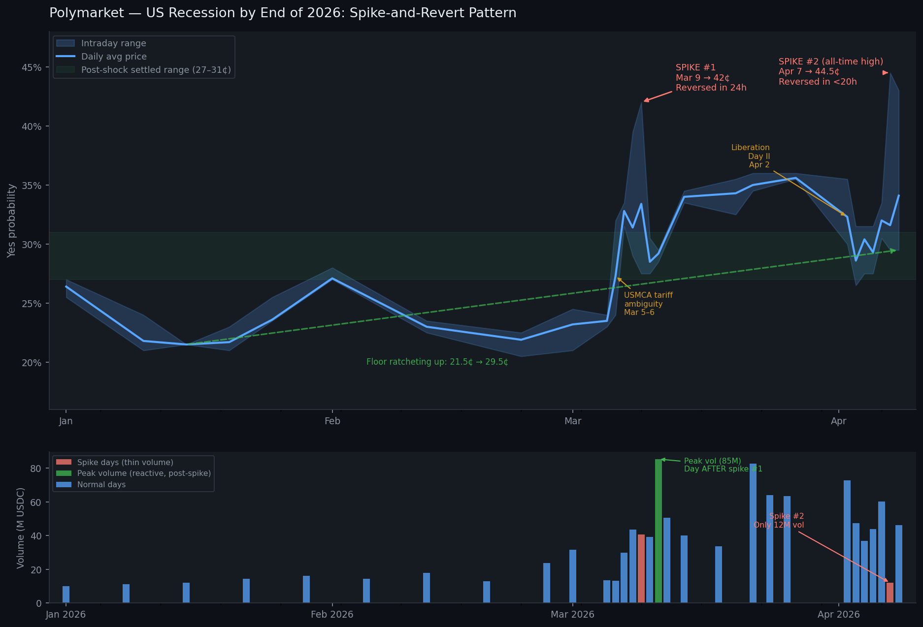
| Date | Avg Price | Intraday High | Event |
|---|---|---|---|
| Jan 15 | 21.5¢ | 21.5¢ | Cycle low (post-inauguration optimism) |
| Mar 5 | 23.5¢ | 23.5¢ | Pre-shock baseline |
| Mar 6 | 27.3¢ | 32.0¢ | Trump tariff policy ambiguity (USMCA exemptions delayed to Apr 2) |
| Mar 7 | 32.8¢ | 33.5¢ | Follow-through |
| Mar 9 | 33.4¢ | 42.0¢ | Spike #1 — thin-book dislocation at 22:00 UTC |
| Mar 10 | 28.5¢ | 30.5¢ | Full reversal (Feb jobs report day — market didn't care) |
| Mar 27 | 35.6¢ | 36.0¢ | New settled range |
| Apr 2 | 32.3¢ | 35.5¢ | Liberation Day II tariff announcement |
| Apr 3 | 28.6¢ | 31.5¢ | Pullback (exemption hopes) |
| Apr 7 | 31.6¢ | 44.5¢ | Spike #2 — all-time high at 22:00 UTC |
| Apr 8 (latest) | ~30¢ | 43.0¢ | Reversal underway (2-week ceasefire announced) |
The two spikes are structurally identical: both exceeded 40¢, both happened near 22:00 UTC, both reversed within 24 hours, and both left the post-reversion price slightly higher than the pre-shock baseline.
The Volume Signal Is the Real Story
If these were informed positioning events — smart money repricing recession risk ahead of the crowd — you'd expect high volume before or during the spike. The data says the opposite.
Using daily volume changes from the market_metrics_history table (cumulative volume is tracked per timestamp, so we diff consecutive days):
| Date | Volume (USDC) | Note |
|---|---|---|
| Jan average | ~10M / day | — |
| Mar 10 | ~39M | First spike day — above normal, but not extreme |
| Mar 11 | ~85M | Single highest volume day in the dataset |
| Apr 6 | ~60M | — |
| Apr 7 | ~12M | Spike to 44.5¢ happened on the lightest day in weeks |
| Apr 8 (partial) | ~40–60M+ (est.) | Traders react to reversal |
March 9's 42¢ spike was followed the next day by the highest-volume session on record (85M). April 7's 44.5¢ spike happened on only 12M volume — less than a typical January day.
The interpretation: these spikes are liquidity events, not information events. A small number of market orders, hitting thin depth at 22:00 UTC, move the price dramatically. Within hours, better-informed (or simply more patient) participants fade the move, and the price snaps back.
If this were fundamental repricing, you'd see volume before the price moved. Instead, volume peaked the day after the March 9 spike — reactive trading, not predictive positioning.
The Ratchet Underneath the Noise
Despite the spikes reversing, the underlying settled price has been trending up all year. Strip out the two spike events and fit a trend through the post-reversion lows:
- Mid-January low: 21.5¢
- Post-March spike floor: ~28.5¢
- Post-April tariff settled range: ~29–31¢
That's a ~9 percentage-point increase in the background recession probability since January — slow, grinding, and entirely invisible if you're only looking at the dramatic intraday moves.
The tariff regime is the driver. Liberation Day II (April 2) imposed a 10% universal baseline with higher reciprocal rates on 60+ countries — the highest average US tariff in a century. J.P. Morgan Research flagged a "large sentiment shock" to business investment as a key recession transmission mechanism. Polymarket's crowd priced this in gradually, not in a single jump: the March 6 move (+8.5¢ in one afternoon), the jobs report absorption (March 10, barely moved), the Liberation Day dip-and-recover — each event left the floor a few cents higher.
The spikes are noise. The ratchet is signal.
What This Looks Like in the Order Book
Bid-ask spread from the market_metrics_history table confirms the thin-liquidity hypothesis. Average spread was 1.5¢ in January. As of late March, it's consistently below 1.1¢ — the market has actually gotten more efficient as trading volume increased. That 44.5¢ print was not a wide-spread, low-quality price. It was a real transaction. It just occurred in a brief window of thin depth that corrected within the hour.
The spread spiking to 1.5¢ on April 8 (up from 1.1¢ the prior week) is consistent with elevated uncertainty while the ceasefire situation resolves.
Reproduce This Analysis
Here's the full Python workflow to pull this data yourself using the polymarketdata.co API:
import os
import pandas as pd
import matplotlib.pyplot as plt
import matplotlib.dates as mdates
from polymarketdata import PolymarketDataClient, Resolution

MARKET_SLUG = "us-recession-by-end-of-2026"

with PolymarketDataClient(api_key=os.environ["POLYMARKETDATA_API_KEY"]) as client:

    # --- Pull daily price data ---
    prices = client.history.get_market_prices(
        MARKET_SLUG,
        start_ts="2026-01-01T00:00:00Z",
        end_ts="2026-04-08T23:59:00Z",
        resolution=Resolution.ONE_HOUR,
    )
    df_prices = prices.to_dataframe_prices()

    # Keep only the "Yes" token (label == "Yes")
    df_yes = df_prices[df_prices["label"] == "Yes"].copy()
    df_yes["t"] = pd.to_datetime(df_yes["t"], utc=True)
    df_yes = df_yes.sort_values("t")

    # Daily OHLC
    df_daily = (
        df_yes.groupby(df_yes["t"].dt.date)["price"]
        .agg(avg="mean", high="max", low="min")
        .reset_index()
        .rename(columns={"t": "date"})
    )

    # --- Pull daily volume + spread ---
    metrics = client.history.get_market_metrics(
        MARKET_SLUG,
        start_ts="2026-01-01T00:00:00Z",
        end_ts="2026-04-08T23:59:00Z",
        resolution=Resolution.ONE_DAY,
    )
    df_metrics = metrics.to_dataframe_metrics()
    df_metrics["t"] = pd.to_datetime(df_metrics["t"], utc=True)

    # Diff cumulative volume to get daily flow
    df_metrics = df_metrics.sort_values("t")
    df_metrics["daily_volume_m"] = df_metrics["volume"].diff() / 1e6

# --- Plot: Price timeline with spike annotations ---
fig, (ax1, ax2) = plt.subplots(2, 1, figsize=(12, 8), sharex=False)
fig.patch.set_facecolor("#0f1117")
for ax in (ax1, ax2):
    ax.set_facecolor("#1a1d27")
    ax.tick_params(colors="white")
    ax.spines[:].set_color("#333")

# Top panel: daily average + intraday high
ax1.fill_between(df_daily["date"], df_daily["low"], df_daily["high"],
                 alpha=0.25, color="#4f8ef7", label="Intraday range")
ax1.plot(df_daily["date"], df_daily["avg"],
         color="#4f8ef7", linewidth=1.8, label="Daily avg")

# Annotate the two spikes
spike1 = df_daily[df_daily["date"].astype(str) == "2026-03-09"]
spike2 = df_daily[df_daily["date"].astype(str) == "2026-04-07"]
for row, label in [(spike1, "Mar 9\n42¢ high"), (spike2, "Apr 7\n44.5¢ high")]:
    if not row.empty:
        ax1.annotate(label, xy=(row["date"].values[0], row["high"].values[0]),
                     xytext=(0, 16), textcoords="offset points",
                     color="#ff6b6b", fontsize=9, ha="center",
                     arrowprops=dict(arrowstyle="-|>", color="#ff6b6b", lw=1.2))

ax1.axhline(0.295, color="#ffd700", linewidth=0.8, linestyle="--", alpha=0.6,
            label="Current settled price (29.5¢)")
ax1.set_ylabel("Yes probability", color="white")
ax1.set_title("Polymarket: US Recession by End of 2026 — Spike-and-Revert Pattern",
              color="white", pad=12)
ax1.legend(loc="upper left", facecolor="#1a1d27", edgecolor="#333",
           labelcolor="white", fontsize=9)
ax1.yaxis.set_major_formatter(plt.FuncFormatter(lambda x, _: f"{x:.0%}"))

# Bottom panel: daily volume
vol_plot = df_metrics.dropna(subset=["daily_volume_m"])
ax2.bar(vol_plot["t"].dt.date, vol_plot["daily_volume_m"],
        color="#4f8ef7", alpha=0.7, width=0.8)
ax2.set_ylabel("Daily volume (M USDC)", color="white")
ax2.set_xlabel("Date", color="white")
ax2.set_title("Daily trading volume — volume LAGGED the March 9 spike by 2 days",
              color="white", pad=8)

plt.tight_layout(pad=2)
plt.savefig("recession_spike_revert.png", dpi=150, bbox_inches="tight",
            facecolor=fig.get_facecolor())
plt.show()
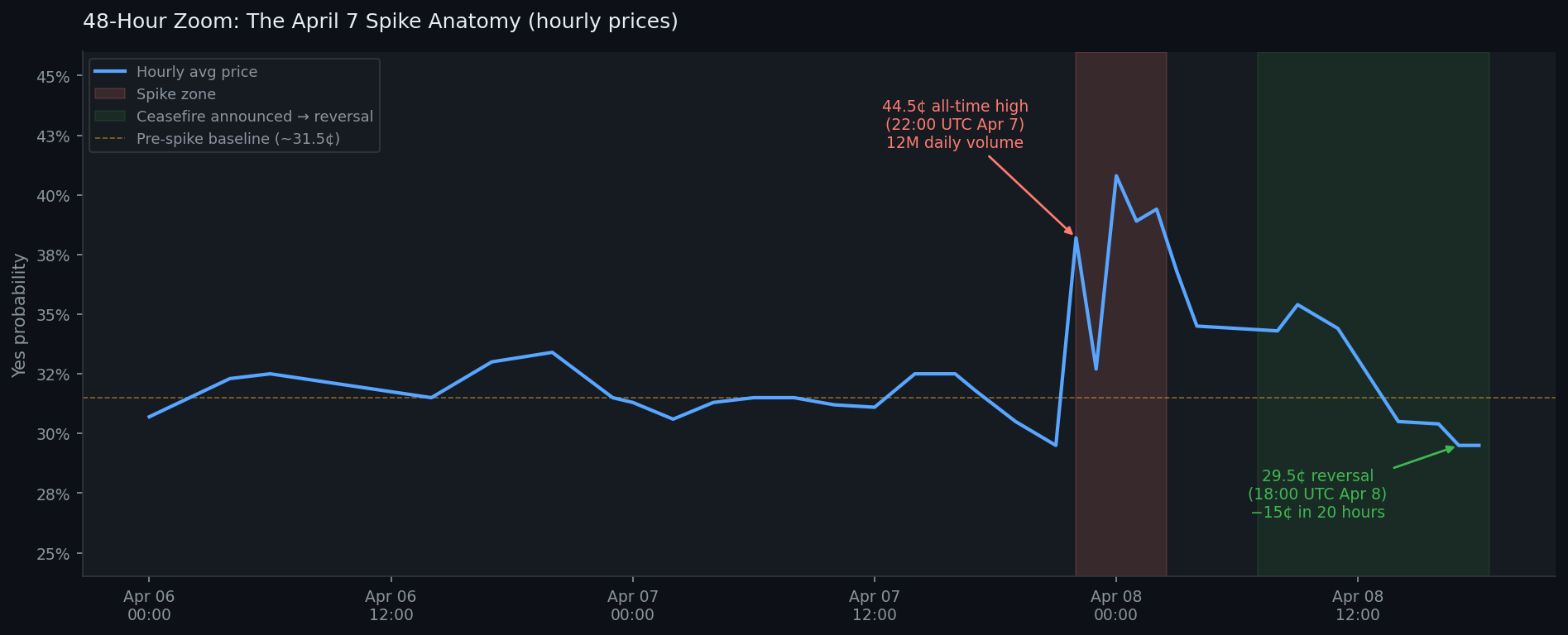
To zoom into just the past 48 hours at 1-minute resolution (this is where you can see the exact shape of the spike-and-revert):
with PolymarketDataClient(api_key=os.environ["POLYMARKETDATA_API_KEY"]) as client:
    prices_1m = client.history.get_market_prices(
        MARKET_SLUG,
        start_ts="2026-04-06T00:00:00Z",
        end_ts="2026-04-08T23:59:00Z",
        resolution=Resolution.ONE_MINUTE,
    )
    df_1m = prices_1m.to_dataframe_prices()
    df_1m = df_1m[df_1m["label"] == "Yes"].copy()
    df_1m["t"] = pd.to_datetime(df_1m["t"], utc=True)

    fig, ax = plt.subplots(figsize=(14, 5))
    ax.plot(df_1m["t"], df_1m["price"], color="#4f8ef7", linewidth=1.2)
    ax.axvline(pd.Timestamp("2026-04-07 22:00:00", tz="UTC"),
               color="#ff6b6b", linewidth=1.2, linestyle="--",
               label="44.5¢ spike (Apr 7 22:00 UTC)")
    ax.axvline(pd.Timestamp("2026-04-08 07:00:00", tz="UTC"),
               color="#ffd700", linewidth=1.2, linestyle="--",
               label="Ceasefire announced — reversal")
    ax.set_title("1-minute prices: Apr 6–8 spike anatomy", color="white")
    ax.yaxis.set_major_formatter(plt.FuncFormatter(lambda x, _: f"{x:.0%}"))
    ax.legend(facecolor="#1a1d27", edgecolor="#333", labelcolor="white")
    plt.tight_layout()
    plt.savefig("recession_48h_zoom.png", dpi=150, bbox_inches="tight")
The Trading Take
Two occurrences is a pattern, not a coincidence. Both 40¢+ prints were at 22:00 UTC; both reversed within 24 hours; both happened on below-average volume.
If you're trading macro markets on Polymarket, the actionable version of this is straightforward: when the recession market spikes 10+ cents intraday on news flow, the order book is temporarily dislocated. The "real" market — where volume-weighted activity has settled the price for days or weeks — hasn't moved. Fading that spike is not a bet against a recession happening; it's a bet that the thin-book price is wrong about where equilibrium sits.
That said, the floor keeps rising. Fading to 30¢ is very different from fading to 21¢. The crowd has genuinely repriced recession risk upward — it's just doing so with a lot of noise layered on top.
The next catalyst is the two-week ceasefire deadline and whether tariff negotiations produce any real exemptions. If neither resolves cleanly, don't be surprised to see a third spike — probably around 22:00 UTC on a low-volume Tuesday.
All data from the polymarketdata.co API. Full endpoint reference at polymarketdata.co/docs.